pacman::p_load(olsrr, corrplot, ggpubr, sf, spdep, GWmodel, tmap, tidyverse, gtsummary,mapview,leaflet,RColorBrewer,tidygeocoder,jsonlite,httr,onemapsgapi,reporter,magrittr,readxl,gdata, units,matrixStats, SpatialML,rsample, Metrics)Take Home Ex 3
Getting Started
In this take-home exercise, you are tasked to predict HDB resale prices at the sub-market level (i.e.HDB 3-room, HDB 4-room and HDB 5-room) for the month of January and February 2023 in Singapore. The predictive models must be built by using by using conventional OLS method and GWR methods. You are also required to compare the performance of the conventional OLS method versus the geographical weighted methods.
The study should focus on either three-room, four-room or five-room flat and transaction period should be from 1st January 2021 to 31st December 2022. The test data should be January and February 2023 resale prices.
The Data
Data sets will be used in this model building exercise, they are:
Loading of packages
Importing Geospatial Data
After I imported the subzone layer and analysed below, I’ve found out that there are some subzone area which can be removed because the area are mostly industrial/campsite and would not have any residents living there.
mpsz19 <- st_read(dsn = "data/geospatial", layer = "MPSZ-2019") %>%
st_transform(3414) %>% filter(SUBZONE_N != "NORTH-EASTERN ISLANDS" & SUBZONE_N != "SOUTHERN GROUP"& SUBZONE_N != "SEMAKAU"& SUBZONE_N != "SUDONG")Reading layer `MPSZ-2019' from data source
`C:\yifei-alpaca\IS415-GAA\Take-home_Ex\Take-home_Ex03\data\geospatial'
using driver `ESRI Shapefile'
Simple feature collection with 332 features and 6 fields
Geometry type: MULTIPOLYGON
Dimension: XY
Bounding box: xmin: 103.6057 ymin: 1.158699 xmax: 104.0885 ymax: 1.470775
Geodetic CRS: WGS 84st_crs(mpsz19)Coordinate Reference System:
User input: EPSG:3414
wkt:
PROJCRS["SVY21 / Singapore TM",
BASEGEOGCRS["SVY21",
DATUM["SVY21",
ELLIPSOID["WGS 84",6378137,298.257223563,
LENGTHUNIT["metre",1]]],
PRIMEM["Greenwich",0,
ANGLEUNIT["degree",0.0174532925199433]],
ID["EPSG",4757]],
CONVERSION["Singapore Transverse Mercator",
METHOD["Transverse Mercator",
ID["EPSG",9807]],
PARAMETER["Latitude of natural origin",1.36666666666667,
ANGLEUNIT["degree",0.0174532925199433],
ID["EPSG",8801]],
PARAMETER["Longitude of natural origin",103.833333333333,
ANGLEUNIT["degree",0.0174532925199433],
ID["EPSG",8802]],
PARAMETER["Scale factor at natural origin",1,
SCALEUNIT["unity",1],
ID["EPSG",8805]],
PARAMETER["False easting",28001.642,
LENGTHUNIT["metre",1],
ID["EPSG",8806]],
PARAMETER["False northing",38744.572,
LENGTHUNIT["metre",1],
ID["EPSG",8807]]],
CS[Cartesian,2],
AXIS["northing (N)",north,
ORDER[1],
LENGTHUNIT["metre",1]],
AXIS["easting (E)",east,
ORDER[2],
LENGTHUNIT["metre",1]],
USAGE[
SCOPE["Cadastre, engineering survey, topographic mapping."],
AREA["Singapore - onshore and offshore."],
BBOX[1.13,103.59,1.47,104.07]],
ID["EPSG",3414]]st_bbox(mpsz19) xmin ymin xmax ymax
2667.538 21448.473 55941.942 50256.334 After plotting a map, we can see that there is an island called NORTH-EASTERN ISLAND, SOUTHERN GROUP, SEMAKAU and SUDONG which is out of analysis area. we should remove them for the purpose of this takehome exercise. We can re-import the data with out this names by doing a filter(). Re run the map and look! its clean now. We can move on to our analysis.
Population Analysis
Importing Aspatial Data Population
In this section, I will be importing Singapore population data. In our Hands-on Ex03 we have use a choropleth map to portray the spatial distribution of aged population of Singapore by Master Plan 2014 Subzone Boundary. Let’s further analyse this data and code further for our analysis.
popdata <- read_csv("data/aspatial/population_2011to2020.csv")popdata2020 <- popdata %>%
filter(Time == 2020) %>%
group_by(PA, SZ, AG) %>%
summarise(`POP` = sum(`Pop`)) %>%
ungroup()%>%
pivot_wider(names_from=AG,
values_from=POP) %>%
mutate(YOUNG = rowSums(.[3:6])
+rowSums(.[12])) %>%
mutate(`ECONOMY ACTIVE` = rowSums(.[7:11])+
rowSums(.[13:15]))%>%
mutate(`AGED`=rowSums(.[16:21])) %>%
mutate(`TOTAL`=rowSums(.[3:21])) %>%
mutate(`DEPENDENCY` = (`YOUNG` + `AGED`)
/`ECONOMY ACTIVE`) %>%
select(`PA`, `SZ`, `YOUNG`,
`ECONOMY ACTIVE`, `AGED`,
`TOTAL`, `DEPENDENCY`)As we look at the raw data, we can create a new data frame to combine the number of population and group by PA and SZ.
Joining the attribute data and geospatial data
For master plan and Pop data frame, there are 2 common variable which we can join them together. PLN_AREA_N = PA & SUBZONE_N = SZ but we have to convert them to upper case first
popdata2020 <- popdata2020 %>%
mutate_at(.vars = vars(PA, SZ),
.funs = funs(toupper)) %>%
filter(`ECONOMY ACTIVE` > 0)left join both master plan and population data by their sub zone level.
mpsz_pop2020 <- left_join(mpsz19, popdata2020,
by = c("SUBZONE_N" = "SZ"))Exploratory Data Analysis (EDA)
tm_shape(mpsz_pop2020)+
tm_fill("DEPENDENCY",
style = "quantile",
palette = "Greens") +
tm_borders(alpha = 0.5)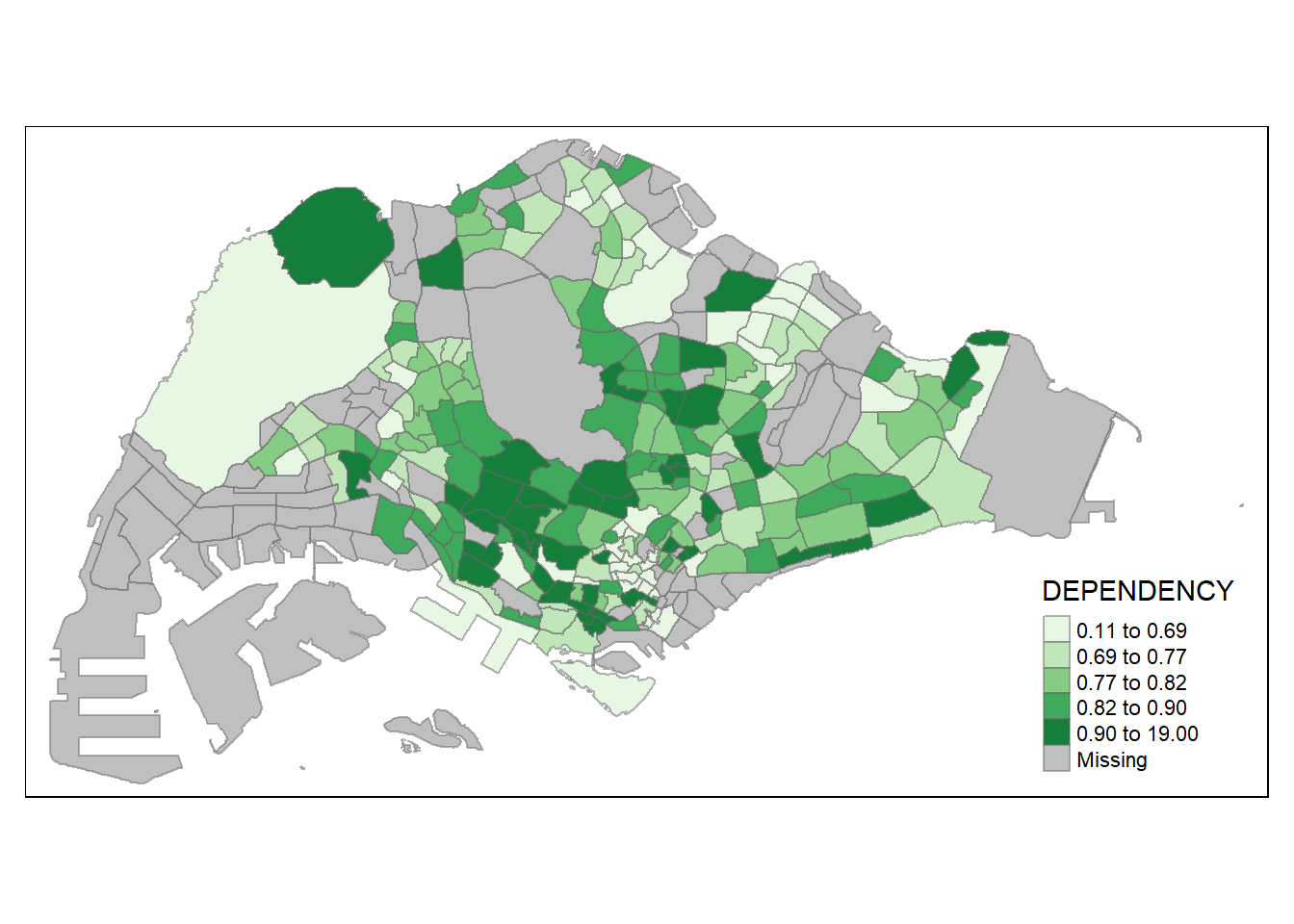
tmap_options(check.and.fix = TRUE)
tm_shape(mpsz_pop2020)+
tm_fill("TOTAL",
style = "quantile",
palette = "Blues") +
tm_borders(alpha = 0.5)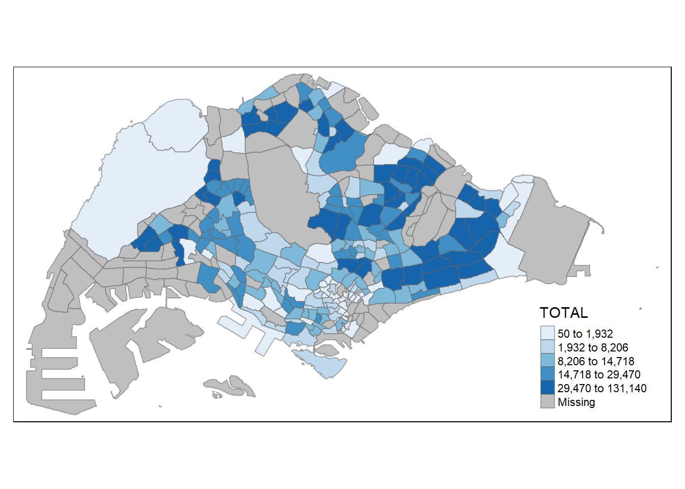
Based on the chart above, we can see that in general, the east area is more dense as compared to the other region.
Lets compare between 3 groups.
tmap_mode("view")tmap_options(check.and.fix = TRUE)
youngmap <- tm_shape(mpsz_pop2020)+
tm_polygons("YOUNG",
style = "quantile",
palette = "Reds",
)+
tm_view(set.zoom.limits = c(9,14))
tmap_options(check.and.fix = TRUE)
activemap <- tm_shape(mpsz_pop2020)+
tm_polygons("ECONOMY ACTIVE",
style = "quantile",
palette = "Blues",
)+
tm_view(set.zoom.limits = c(9,14))
agedmap <- tm_shape(mpsz_pop2020)+
tm_polygons("AGED",
style = "quantile",
palette = "Oranges") +
tm_view(set.zoom.limits = c(9,14))
tmap_arrange(youngmap,activemap, agedmap, asp=1, ncol=3, sync = TRUE)tmap_mode("plot")Based on the interactive graph above, we can say that the east area has a more dense aged group as compared to the economy active group. In general, I can also say that; the east area has a higher aging population as compared to other areas. Furthermore, we can also conclude that there are more resident staying in the east side than other region.
Existing Dwelling Analysis
Notice that in the excel sheet, there is a column called dwelling as shown below. We can also further analysis the current type of dwelling to narrow down which type of housing are most common/popular.
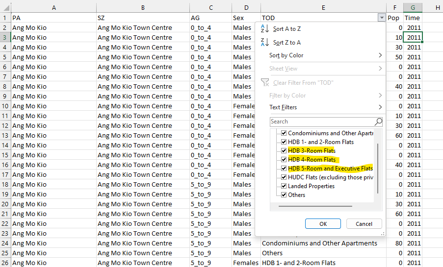
dwelling2020 <- popdata %>%
filter(Time == 2020 &
TOD == "HDB 3-Room Flats" |
TOD == "HDB 4-Room Flats" |
TOD == "HDB 5-Room and Executive Flats") %>%
group_by(PA, SZ, TOD) %>%
summarise(`POP` = sum(`Pop`))Joining the attribute data and geospatial data
dwelling2020 <- dwelling2020 %>%
mutate_at(.vars = vars(PA, SZ),
.funs = funs(toupper)) %>%
filter(`POP` > 0)mpsz_dwelling2020 <- left_join(mpsz19, dwelling2020,
by = c("SUBZONE_N" = "SZ"))Exploratory Data Analysis (EDA)
tmap_mode("view")
HDB3room <- tm_shape(mpsz_dwelling2020 %>% filter( TOD == "HDB 3-Room Flats"))+
tm_fill("POP",
style = "quantile",
palette = "Greens") +
tm_view(set.zoom.limits = c(10,14))
HDB4room <- tm_shape(mpsz_dwelling2020 %>% filter( TOD == "HDB 4-Room Flats"))+
tm_polygons("POP",
style = "quantile",
palette = "Blues",
)+
tm_view(set.zoom.limits = c(10,14))
HDB5room <- tm_shape(mpsz_dwelling2020 %>% filter( TOD == "HDB 5-Room and Executive Flats"))+
tm_polygons("POP",
style = "quantile",
palette = "Reds") +
tm_view(set.zoom.limits = c(10,14))
tmap_arrange(HDB3room, HDB4room, HDB5room, asp=1, ncol=3, sync = TRUE)Mentioned above that the study should focus on either three-room, four-room or five-room flat. Based on the chart above, we can see that 4-room flat has a higher results as compared to 3-room and 5-room due to its scale of 536,920 for 4-room, next highest is 495,380 for 5-room and 30,880 for 3-room. With this dwelling analysis, I will be focusing on 4-Room flat cause of its popularity in Singapore.
Importing Locational factors
The data mostly are taken from data.gov or LTA data mall factors include:
Bus stop location LTA data mall
Eldercare data.gov
Foodarea
schools data.gov
childcare (taken from our inclass exercise)
train station kaggel
malls from kaggle
supermarket geofabrik
hospital (collated manually) SGhospital
As there are many views about elite schools in Singapore as attending an elite primary school in Singapore is important depends on an individual’s unique circumstances and goals. In this take home exercise, I will be picking the top 10 most common popular primary schools. These are the top 10 popular schools according to this website.
busstops <- st_read(dsn = "data/aspatial/BusStopLocation", layer = "BusStop")Reading layer `BusStop' from data source
`C:\yifei-alpaca\IS415-GAA\Take-home_Ex\Take-home_Ex03\data\aspatial\BusStopLocation'
using driver `ESRI Shapefile'
Simple feature collection with 5159 features and 3 fields
Geometry type: POINT
Dimension: XY
Bounding box: xmin: 3970.122 ymin: 26482.1 xmax: 48284.56 ymax: 52983.82
Projected CRS: SVY21eldercare <- st_read(dsn = "data/aspatial/eldercare-services-shp", layer = "ELDERCARE")Reading layer `ELDERCARE' from data source
`C:\yifei-alpaca\IS415-GAA\Take-home_Ex\Take-home_Ex03\data\aspatial\eldercare-services-shp'
using driver `ESRI Shapefile'
Simple feature collection with 133 features and 18 fields
Geometry type: POINT
Dimension: XY
Bounding box: xmin: 14481.92 ymin: 28218.43 xmax: 41665.14 ymax: 46804.9
Projected CRS: SVY21poi <- st_read(dsn = "data/aspatial/poi_singapore", layer = "Singapore_POIS")Reading layer `Singapore_POIS' from data source
`C:\yifei-alpaca\IS415-GAA\Take-home_Ex\Take-home_Ex03\data\aspatial\poi_singapore'
using driver `ESRI Shapefile'
Simple feature collection with 18687 features and 4 fields
Geometry type: POINT
Dimension: XY
Bounding box: xmin: 3699.08 ymin: 22453.07 xmax: 52883.86 ymax: 50153.8
Projected CRS: SVY21 / Singapore TMAfter we see the poi datafame, lets check for unique values under fclass
unique(poi$fclass) [1] "bakery" "viewpoint" "atm"
[4] "attraction" "toilet" "fast_food"
[7] "convenience" "supermarket" "food_court"
[10] "bank" "post_office" "restaurant"
[13] "cafe" "monument" "shelter"
[16] "tourist_info" "bench" "college"
[19] "telephone" "memorial" "bar"
[22] "pub" "pharmacy" "cinema"
[25] "theatre" "department_store" "school"
[28] "playground" "water_tower" "fire_station"
[31] "vending_any" "dentist" "post_box"
[34] "stadium" "hospital" "police"
[37] "recycling" "artwork" "camera_surveillance"
[40] "library" "car_dealership" "laundry"
[43] "observation_tower" "lighthouse" "sports_centre"
[46] "fountain" "gift_shop" "doityourself"
[49] "toy_shop" "florist" "hairdresser"
[52] "clothes" "beverages" "jeweller"
[55] "vending_machine" "kindergarten" "greengrocer"
[58] "butcher" "battlefield" "museum"
[61] "waste_basket" "pitch" "community_centre"
[64] "drinking_water" "clinic" "market_place"
[67] "general" "picnic_site" "bookshop"
[70] "travel_agent" "camp_site" "embassy"
[73] "town_hall" "doctors" "bicycle_rental"
[76] "zoo" "bicycle_shop" "comms_tower"
[79] "tower" "guesthouse" "nightclub"
[82] "university" "computer_shop" "sports_shop"
[85] "arts_centre" "swimming_pool" "furniture_shop"
[88] "theme_park" "veterinary" "beauty_shop"
[91] "outdoor_shop" "video_shop" "ice_rink"
[94] "motel" "public_building" "car_rental"
[97] "stationery" "newsagent" "chemist"
[100] "mobile_phone_shop" "ruins" "hotel"
[103] "park" "shoe_shop" "optician"
[106] "mall" "hostel" "car_wash"
[109] "kiosk" "chalet" "water_well"
[112] "prison" "wayside_shrine" "recycling_paper"
[115] "wayside_cross" "car_sharing" "garden_centre"
[118] "recycling_glass" "dog_park" We notice that there are a lot of category, lets only select supermarket for our analysis as there are some inaccuracy in certain classes.
supermarkets <- st_read(dsn = "data/aspatial/poi_singapore", layer = "Singapore_POIS") %>%
filter(fclass == "supermarket")Reading layer `Singapore_POIS' from data source
`C:\yifei-alpaca\IS415-GAA\Take-home_Ex\Take-home_Ex03\data\aspatial\poi_singapore'
using driver `ESRI Shapefile'
Simple feature collection with 18687 features and 4 fields
Geometry type: POINT
Dimension: XY
Bounding box: xmin: 3699.08 ymin: 22453.07 xmax: 52883.86 ymax: 50153.8
Projected CRS: SVY21 / Singapore TMfoodarea <- st_read(dsn = "data/aspatial/poi_singapore", layer = "Singapore_POIS") %>%
filter(fclass == "food_court"| fclass == "fast_food"
|fclass =="restaurant" |fclass =="cafe")Reading layer `Singapore_POIS' from data source
`C:\yifei-alpaca\IS415-GAA\Take-home_Ex\Take-home_Ex03\data\aspatial\poi_singapore'
using driver `ESRI Shapefile'
Simple feature collection with 18687 features and 4 fields
Geometry type: POINT
Dimension: XY
Bounding box: xmin: 3699.08 ymin: 22453.07 xmax: 52883.86 ymax: 50153.8
Projected CRS: SVY21 / Singapore TMtrainstation <- read_csv("data/aspatial/mrt_lrt_data.csv")childcare <- st_read(dsn = "data/aspatial", layer = "ChildcareServices")Reading layer `ChildcareServices' from data source
`C:\yifei-alpaca\IS415-GAA\Take-home_Ex\Take-home_Ex03\data\aspatial'
using driver `ESRI Shapefile'
Simple feature collection with 1545 features and 2 fields
Geometry type: POINT
Dimension: XYZ
Bounding box: xmin: 11203.01 ymin: 25667.6 xmax: 45404.24 ymax: 49300.88
z_range: zmin: 0 zmax: 0
Projected CRS: SVY21 / Singapore TMhospital <- read_excel("data/aspatial/hospital.xlsx")good_prischool <- read_csv("data/aspatial/school-directory-and-information/general-information-of-schools.csv") %>% filter(
school_name == "NANYANG PRIMARY SCHOOL" |
school_name == "CATHOLIC HIGH SCHOOL" |
school_name == "TAO NAN SCHOOL" |
school_name == "NAN HUA PRIMARY SCHOOL" |
school_name == "ST. HILDA'S PRIMARY SCHOOL" |
school_name == "HENRY PARK PRIMARY SCHOOL" |
school_name == "ANGLO-CHINESE SCHOOL (PRIMARY)" |
school_name == "RAFFLES GIRLS' PRIMARY SCHOOL" |
school_name == "PEI HWA PRESBYTERIAN PRIMARY SCHOOL" |
school_name == "CHIJ ST. NICHOLAS GIRLS' SCHOOL")primaryschool <- read_csv("data/aspatial/school-directory-and-information/general-information-of-schools.csv") %>% filter(mainlevel_code =="PRIMARY")shoppingmalls <- read_csv("data/aspatial/shopping_mall_coordinates.csv")Change dataframe to sf format
busstop.sf <- st_transform(busstops, crs=3414)
eldercare.sf <- st_transform(eldercare, crs=3414)
foodarea.sf <- st_transform(foodarea, crs=3414)
supermarkets.sf <- st_transform(supermarkets, crs=3414)
childcare.sf <- st_transform(childcare, crs=3414)
hospital.sf <- st_as_sf(hospital,
coords = c("Long", "Lat"),
crs=4326) %>%
st_transform(crs=3414)
trainstation.sf <- st_as_sf(trainstation,
coords = c("lng", "lat"),
crs=4326) %>%
st_transform(crs=3414)We note that there are no Lat and Long in the primary school data frame. we need to tidy the data for both primary and good primary schools. To prevent it from rendering the website for too long, I will be exporting and importing the tidied files.
# primaryschool[c('block', 'street')] <- str_split_fixed(primaryschool$address, ' ', # 2)
# primaryschool$street<- trim(primaryschool$street)
# primaryschool$street<- toupper(primaryschool$street)# good_prischool[c('block', 'street')] <- str_split_fixed(good_prischool$address, ' '# , 2)
# good_prischool$street<- trim(good_prischool$street)
# good_prischool$street<- toupper(good_prischool$street)#library(httr)
#geocode <- function(block, streetname) {
# base_url <- "https://developers.onemap.sg/commonapi/search"
# address <- paste(block, streetname, sep = " ")
# query <- list("searchVal" = address,
# "returnGeom" = "Y",
# "getAddrDetails" = "N",
# "pageNum" = "1")
#
# res <- GET(base_url, query = query)
# restext<-content(res, as="text")
#
# output <- fromJSON(restext) %>%
# as.data.frame %>%
# select(results.LATITUDE, results.LONGITUDE)
#
# return(output)
#}#good_prischool$LATITUDE <- 0
#good_prischool$LONGITUDE <- 0
#
#for (i in 1:nrow(good_prischool)){
# temp_output <- geocode(good_prischool[i, 32], good_prischool[i, 33])
#
# good_prischool$LATITUDE[i] <- temp_output$results.LATITUDE
# good_prischool$LONGITUDE[i] <- temp_output$results.LONGITUDE
#}# primaryschool$LATITUDE <- 0
# primaryschool$LONGITUDE <- 0
#
# for (i in 1:nrow(primaryschool)){
# temp_output <- geocode(primaryschool[i, 32], primaryschool[i, 33])
#
# primaryschool$LATITUDE[i] <- temp_output$results.LATITUDE
# primaryschool$LONGITUDE[i] <- temp_output$results.LONGITUDE
# }Export tidy data for schools
#write.csv(primaryschool,"data/exported/primaryschool.csv")
#write.csv(good_prischool,"data/exported/good_prischool.csv")Import tidy data for schools
primaryschool <- read_csv("data/exported/primaryschool.csv")
good_prischool <- read_csv("data/exported/good_prischool.csv")After we have done, we can proceed to convert the df to sf.
shoppingmalls.sf <- st_as_sf(shoppingmalls,
coords = c("LONGITUDE", "LATITUDE"),
crs=4326) %>%
st_transform(crs=3414)
good_prischool.sf <- st_as_sf(good_prischool,
coords = c("LONGITUDE", "LATITUDE"),
crs=4326) %>%
st_transform(crs=3414)
primaryschool.sf <- st_as_sf(primaryschool,
coords = c("LONGITUDE", "LATITUDE"),
crs=4326) %>%
st_transform(crs=3414)Exploratory Data Analysis (EDA)
tmap_mode("plot")
PLOT_BUS <- tm_shape(mpsz19) +
tm_borders(alpha = 0.5) +
tmap_options(check.and.fix = TRUE) +
tm_shape(busstop.sf) +
tm_dots(col="red", size=0.05) +
tm_layout(main.title = "Bus Stops",
main.title.position = "center",
main.title.size = 1.2,
frame = TRUE)+
tm_view(set.zoom.limits = c(10,14))
PLOT_TRAIN <- tm_shape(mpsz19) +
tm_borders(alpha = 0.5) +
tmap_options(check.and.fix = TRUE) +
tm_shape(trainstation.sf) +
tm_dots(col="blue", size=0.05) +
tm_layout(main.title = "Train Station",
main.title.position = "center",
main.title.size = 1.2,
frame = TRUE)+
tm_view(set.zoom.limits = c(10,14))
tmap_arrange(PLOT_BUS, PLOT_TRAIN,
asp=1, ncol=2,
sync = FALSE)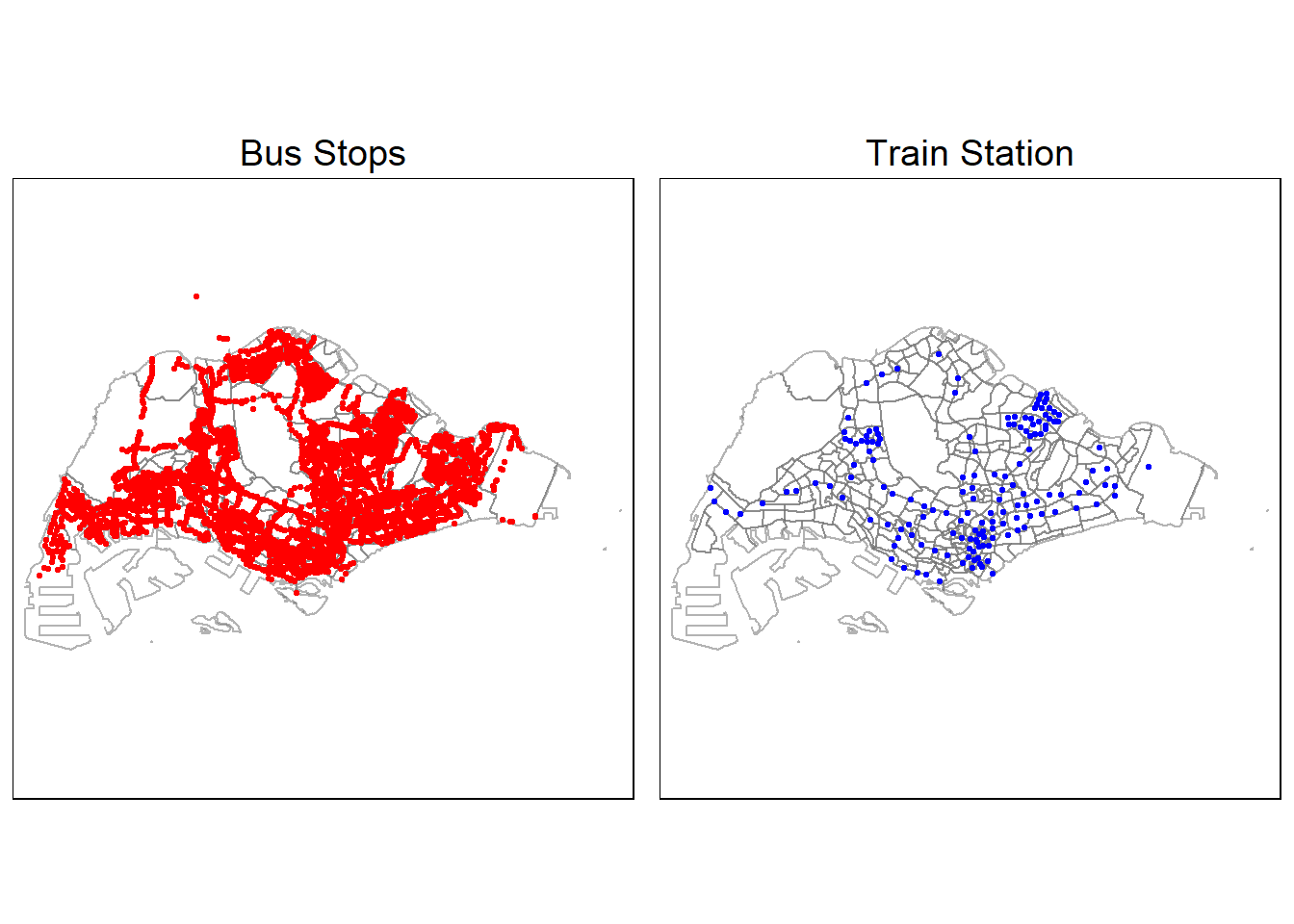
Notice for bus stop, there are a few points that is out of Singapore, lets remove those points namely “LARKIN TER”, “KOTARAYA II TER”, “JOHOR BAHRU CHECKPT”, “JB SENTRAL”. After that, we can re-run the map above.
busstop.sf <- busstop.sf %>%
filter(LOC_DESC != "JOHOR BAHRU CHECKPT" & LOC_DESC != "LARKIN TER"& LOC_DESC != "KOTARAYA II TER"& LOC_DESC != "JB SENTRAL")Lets looks at other data.
tmap_mode("plot")
PLOT_CHILD <- tm_shape(mpsz19) +
tm_borders(alpha = 0.5) +
tmap_options(check.and.fix = TRUE) +
tm_shape(childcare.sf) +
tm_dots(col="orange", size=0.05) +
tm_layout(main.title = "Child Care",
main.title.position = "center",
main.title.size = 1.2,
frame = TRUE)+
tm_view(set.zoom.limits = c(10,14))
PLOT_ELDER <- tm_shape(mpsz19) +
tm_borders(alpha = 0.5) +
tmap_options(check.and.fix = TRUE) +
tm_shape(eldercare.sf) +
tm_dots(col="green", size=0.05) +
tm_layout(main.title = "Elder Care",
main.title.position = "center",
main.title.size = 1.2,
frame = TRUE)+
tm_view(set.zoom.limits = c(10,14))
tmap_arrange(PLOT_CHILD, PLOT_ELDER,
asp=1, ncol=2,
sync = FALSE)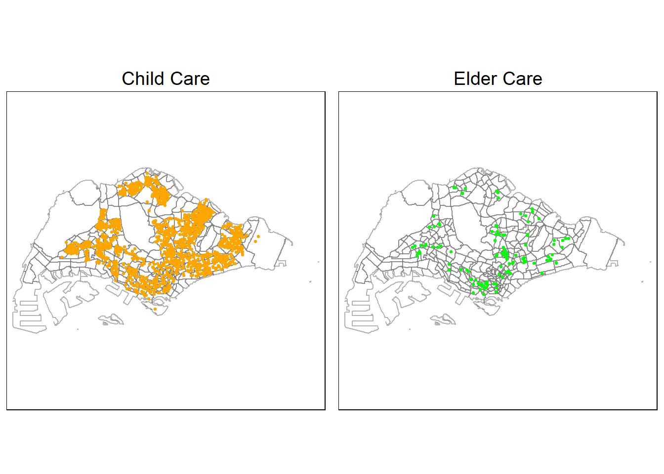
tmap_mode("plot")
PLOT_PRISCHOOL <- tm_shape(mpsz19) +
tm_borders(alpha = 0.5) +
tmap_options(check.and.fix = TRUE) +
tm_shape(primaryschool.sf) +
tm_dots(col="#009999", size=0.05) +
tm_layout(main.title = "Primary school",
main.title.position = "center",
main.title.size = 1.2,
frame = TRUE)+
tm_view(set.zoom.limits = c(10,14))
PLOT_GOODPRISCHOOL <- tm_shape(mpsz19) +
tm_borders(alpha = 0.5) +
tmap_options(check.and.fix = TRUE) +
tm_shape(good_prischool.sf) +
tm_dots(col="red", size=0.05) +
tm_layout(main.title = "Good Primary School",
main.title.position = "center",
main.title.size = 1.2,
frame = TRUE)+
tm_view(set.zoom.limits = c(10,14))
tmap_arrange(PLOT_PRISCHOOL, PLOT_GOODPRISCHOOL,
asp=1, ncol=2,
sync = FALSE)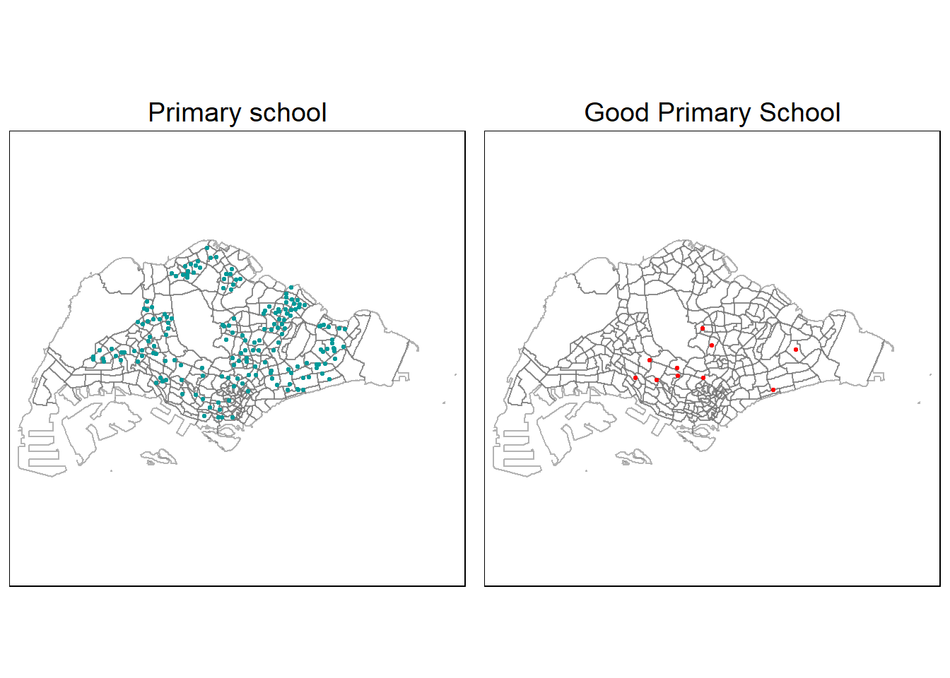
tmap_mode("plot")
PLOT_FOOD <- tm_shape(mpsz19) +
tm_borders(alpha = 0.5) +
tmap_options(check.and.fix = TRUE) +
tm_shape(foodarea.sf) +
tm_dots(col="#009999", size=0.05) +
tm_layout(main.title = "Food Area",
main.title.position = "center",
main.title.size = 1.2,
frame = TRUE)+
tm_view(set.zoom.limits = c(10,14))
PLOT_SUPERMART <- tm_shape(mpsz19) +
tm_borders(alpha = 0.5) +
tmap_options(check.and.fix = TRUE) +
tm_shape(supermarkets.sf) +
tm_dots(col="#0000FF", size=0.05) +
tm_layout(main.title = "Supermarket",
main.title.position = "center",
main.title.size = 1.2,
frame = TRUE)+
tm_view(set.zoom.limits = c(10,14))
tmap_arrange(PLOT_FOOD, PLOT_SUPERMART,
asp=1, ncol=2,
sync = FALSE)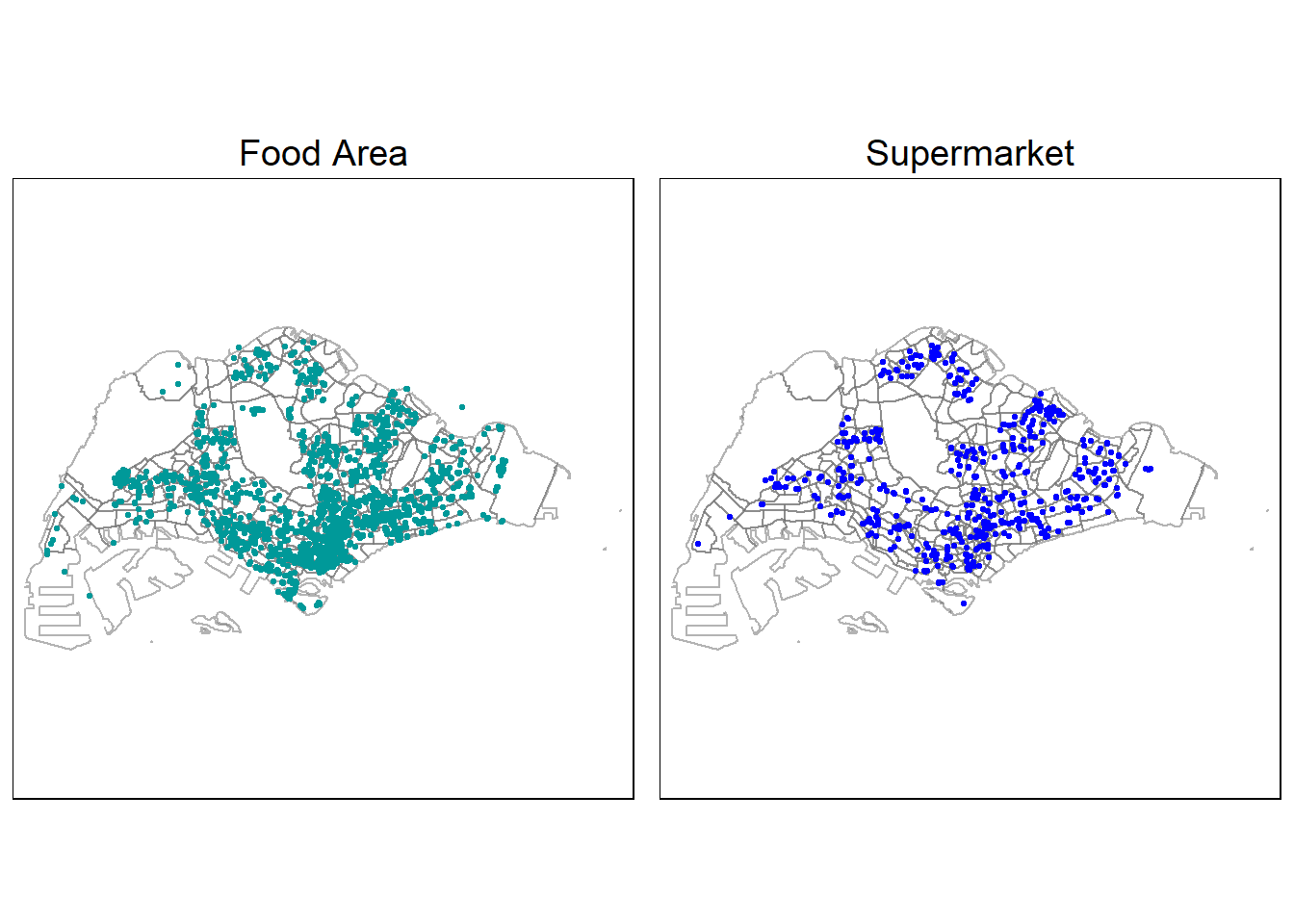
After plotting, we saw a point which is not within SG, let’s remove them and re run the map.
foodarea.sf <- foodarea.sf %>%
filter(osm_id != "4493618264")tmap_mode("plot")
PLOT_HOST <- tm_shape(mpsz19) +
tm_borders(alpha = 0.5) +
tmap_options(check.and.fix = TRUE) +
tm_shape(hospital.sf) +
tm_dots(col="red", size=0.05) +
tm_layout(main.title = "Hospital",
main.title.position = "center",
main.title.size = 1.2,
frame = TRUE)+
tm_view(set.zoom.limits = c(10,14))
PLOT_MALL <- tm_shape(mpsz19) +
tm_borders(alpha = 0.5) +
tmap_options(check.and.fix = TRUE) +
tm_shape(shoppingmalls.sf) +
tm_dots(col="orange", size=0.05) +
tm_layout(main.title = "Shopping mall",
main.title.position = "center",
main.title.size = 1.2,
frame = TRUE)+
tm_view(set.zoom.limits = c(10,14))
tmap_arrange(PLOT_HOST, PLOT_MALL,
asp=1, ncol=2,
sync = FALSE)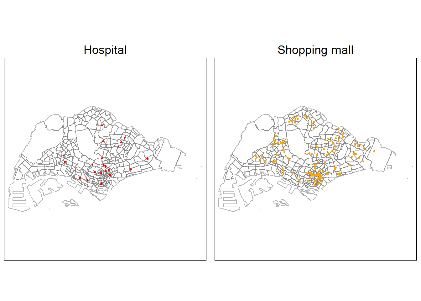
Looks like all data points are within Singapore! Next, we will be preparing data for the HDB resale price.
Importing Aspatial Data HDB resale price
We will import the HDB resale prices and also filter the data to 4-room flat from 1st January 2021 to 31st December 2022 fro training purposes
hdb_resale <- read_csv("data/aspatial/resale_flat_price_full.csv") %>%
filter(flat_type == "4 ROOM") %>%
filter(month >= "2021-01" & month <= "2022-12")glimpse(hdb_resale)Rows: 23,656
Columns: 11
$ month <chr> "2021-01", "2021-01", "2021-01", "2021-01", "2021-…
$ town <chr> "ANG MO KIO", "ANG MO KIO", "ANG MO KIO", "ANG MO …
$ flat_type <chr> "4 ROOM", "4 ROOM", "4 ROOM", "4 ROOM", "4 ROOM", …
$ block <chr> "547", "414", "509", "467", "571", "134", "204", "…
$ street_name <chr> "ANG MO KIO AVE 10", "ANG MO KIO AVE 10", "ANG MO …
$ storey_range <chr> "04 TO 06", "01 TO 03", "01 TO 03", "07 TO 09", "0…
$ floor_area_sqm <dbl> 92, 92, 91, 92, 92, 98, 92, 92, 92, 92, 92, 109, 9…
$ flat_model <chr> "New Generation", "New Generation", "New Generatio…
$ lease_commence_date <dbl> 1981, 1979, 1980, 1979, 1979, 1978, 1977, 1978, 19…
$ remaining_lease <chr> "59 years", "57 years 09 months", "58 years 06 mon…
$ resale_price <dbl> 370000, 375000, 380000, 385000, 410000, 410000, 41…Next, we will be importing test data. The test data should be January and February 2023 resale prices. We will be filtering January to Feb 2023 and 4-room flat.
hdb_resale_test <- read_csv("data/aspatial/resale_flat_price_full.csv") %>%
filter(flat_type == "4 ROOM") %>%
filter(month >= "2023-01" & month <= "2023-02")In the below data prep, we should clean the data for both test and train.
Data Preparation
Since there is no Long and Lat in the data, we need to create one. But before that we can combine the block with the street name, create category column representing story range, create Lat Long column and reformat remaining lease.
- Combine block and street name
hdb_resale$address <- paste(hdb_resale$block, hdb_resale$street_name, sep=" ")hdb_resale_test$address <- paste(hdb_resale_test$block, hdb_resale_test$street_name, sep=" ")- Looking at megan’s Takehome, she created duplicate values representing the story range. I was thinking of something different, so I decided we can categories in 4 category Low, Mid, High, very High instead.
Low: 01-06
Middle: 07-12
High: 13-24
Very High: >= 25
unique(hdb_resale$storey_range) [1] "04 TO 06" "01 TO 03" "07 TO 09" "10 TO 12" "13 TO 15" "16 TO 18"
[7] "19 TO 21" "22 TO 24" "28 TO 30" "25 TO 27" "31 TO 33" "43 TO 45"
[13] "34 TO 36" "37 TO 39" "40 TO 42" "46 TO 48" "49 TO 51"Low
hdb_resale$story_level_low <- ifelse(hdb_resale$storey_range=="01 TO 03"|hdb_resale$storey_range=="04 TO 06", 1, 0)hdb_resale_test$story_level_low <- ifelse(hdb_resale_test$storey_range=="01 TO 03"|hdb_resale_test$storey_range=="04 TO 06", 1, 0)Middle
hdb_resale$story_level_mid <- ifelse(hdb_resale$storey_range=="07 TO 09"|hdb_resale$storey_range=="10 TO 12", 1, 0)hdb_resale_test$story_level_mid <- ifelse(hdb_resale_test$storey_range=="07 TO 09"|hdb_resale_test$storey_range=="10 TO 12", 1, 0)High
hdb_resale$story_level_high <- ifelse(hdb_resale$storey_range=="13 TO 15"|hdb_resale$storey_range=="16 TO 18"|hdb_resale$storey_range=="19 TO 21"|hdb_resale$storey_range=="22 TO 24", 1, 0)hdb_resale_test$story_level_high <- ifelse(hdb_resale_test$storey_range=="13 TO 15"|hdb_resale_test$storey_range=="16 TO 18"|hdb_resale_test$storey_range=="19 TO 21"|hdb_resale_test$storey_range=="22 TO 24", 1, 0)Very High
hdb_resale$story_level_veryhigh <- ifelse(hdb_resale$storey_range>="25 TO 27", 1, 0)hdb_resale_test$story_level_veryhigh <- ifelse(hdb_resale_test$storey_range>="25 TO 27", 1, 0)- Create Lat Long column
The below code, i have copied the from our senior Megan website. The below code extracts the Latitude and Longitude of the address through OneMap API. I have commented after I ran the code once, the process took me about 1 hour to finish extracting the longlat.
I will be exporting it into XLSX file and read in the file.
#library(httr)
#geocode <- function(block, streetname) {
# base_url <- "https://developers.onemap.sg/commonapi/search"
# address <- paste(block, streetname, sep = " ")
# query <- list("searchVal" = address,
# "returnGeom" = "Y",
# "getAddrDetails" = "N",
# "pageNum" = "1")
#
# res <- GET(base_url, query = query)
# restext<-content(res, as="text")
#
# output <- fromJSON(restext) %>%
# as.data.frame %>%
# select(results.LATITUDE, results.LONGITUDE)
#
# return(output)
#}#hdb_resale$LATITUDE <- 0
#hdb_resale$LONGITUDE <- 0
#
#for (i in 1:nrow(hdb_resale)){
# temp_output <- geocode(hdb_resale[i, 4], hdb_resale[i, 5])
#
# hdb_resale$LATITUDE[i] <- temp_output$results.LATITUDE
# hdb_resale$LONGITUDE[i] <- temp_output$results.LONGITUDE
#}#hdb_resale_test$LATITUDE <- 0
#hdb_resale_test$LONGITUDE <- 0
#
#for (i in 1:nrow(hdb_resale_test)){
# temp_output <- geocode(hdb_resale_test[i, 4], hdb_resale_test[i,5])
#
# hdb_resale_test$LATITUDE[i] <- temp_output$results.LATITUDE
# hdb_resale_test$LONGITUDE[i] <- temp_output$results.LONGITUDE
#}#write.csv(hdb_resale,"data/exported/hdb_resale_latlong.csv")#write.csv(hdb_resale_test,"data/exported/hdb_resale_test_latlong.csv")Read in the hdb resale price with latlong column.
hdb_resale <- read_csv("data/exported/hdb_resale_latlong.csv")
hdb_resale_test <- read_csv("data/exported/hdb_resale_test_latlong.csv")Lets check for any NA values
sum(is.na(hdb_resale$LATITUDE))[1] 0sum(is.na(hdb_resale$LONGITUDE))[1] 0sum(is.na(hdb_resale_test$LATITUDE))[1] 0sum(is.na(hdb_resale_test$LONGITUDE))[1] 0There is no missing value and we can proceed to the next steps.
- Convert Remaining lease format
str_list <- str_split(hdb_resale$remaining_lease, " ")
for (i in 1:length(str_list)) {
if (length(unlist(str_list[i])) > 2) {
year <- as.numeric(unlist(str_list[i])[1])
month <- as.numeric(unlist(str_list[i])[3])
hdb_resale$remaining_lease[i] <- year + round(month/12, 2)
}
else {
year <- as.numeric(unlist(str_list[i])[1])
hdb_resale$remaining_lease[i] <- year
}
}
str_list <- str_split(hdb_resale_test$remaining_lease, " ")
for (i in 1:length(str_list)) {
if (length(unlist(str_list[i])) > 2) {
year <- as.numeric(unlist(str_list[i])[1])
month <- as.numeric(unlist(str_list[i])[3])
hdb_resale_test$remaining_lease[i] <- year + round(month/12, 2)
}
else {
year <- as.numeric(unlist(str_list[i])[1])
hdb_resale_test$remaining_lease[i] <- year
}
}Converting aspatial data dataframe into a sf object.
Currently, the hdb_resale tibble data frame is aspatial. We will convert it to a sf object and the output will be in point feature form. The code chunk below converts hdb_resale data frame into a simple feature data frame by using st_as_sf() of sf packages.
hdb_resale.sf <- st_as_sf(hdb_resale,
coords = c("LONGITUDE", "LATITUDE"),
crs=4326) %>%
st_transform(crs=3414)
hdb_resale_test.sf <- st_as_sf(hdb_resale_test,
coords = c("LONGITUDE", "LATITUDE"),
crs=4326) %>%
st_transform(crs=3414)head(hdb_resale.sf)Simple feature collection with 6 features and 17 fields
Geometry type: POINT
Dimension: XY
Bounding box: xmin: 28960.32 ymin: 38439.17 xmax: 30770.07 ymax: 39578.64
Projected CRS: SVY21 / Singapore TM
# A tibble: 6 × 18
...1 month town flat_…¹ block stree…² store…³ floor…⁴ flat_…⁵ lease…⁶
<dbl> <chr> <chr> <chr> <chr> <chr> <chr> <dbl> <chr> <dbl>
1 1 2021-01 ANG MO KIO 4 ROOM 547 ANG MO… 04 TO … 92 New Ge… 1981
2 2 2021-01 ANG MO KIO 4 ROOM 414 ANG MO… 01 TO … 92 New Ge… 1979
3 3 2021-01 ANG MO KIO 4 ROOM 509 ANG MO… 01 TO … 91 New Ge… 1980
4 4 2021-01 ANG MO KIO 4 ROOM 467 ANG MO… 07 TO … 92 New Ge… 1979
5 5 2021-01 ANG MO KIO 4 ROOM 571 ANG MO… 07 TO … 92 New Ge… 1979
6 6 2021-01 ANG MO KIO 4 ROOM 134 ANG MO… 07 TO … 98 New Ge… 1978
# … with 8 more variables: remaining_lease <chr>, resale_price <dbl>,
# address <chr>, story_level_low <dbl>, story_level_mid <dbl>,
# story_level_high <dbl>, story_level_veryhigh <dbl>, geometry <POINT [m]>,
# and abbreviated variable names ¹flat_type, ²street_name, ³storey_range,
# ⁴floor_area_sqm, ⁵flat_model, ⁶lease_commence_dateLet’s visualize the 4-room price in a map view.
tmap_mode("view")
tmap_options(check.and.fix = TRUE)
tm_shape(hdb_resale.sf) +
tm_dots(col = "resale_price",
alpha = 0.6,
style="quantile") +
tm_view(set.zoom.limits = c(11,14))