pacman::p_load(sf, tidyverse, funModeling)In-Class Ex02
Getting started
Download 3 R packages:
Notes to take note of:
st_ refers to spatial and temporal
sf, the table with feature attributes and feature geometries, which contains
sfc , the list-column with the geometries for each feature (record), which is composed of
sfg, the feature geometry of an individual simple feature.
Importing Geospatial
The geoBoundaries dataset
geoNGA <- st_read("data/geospatial/",
                  layer = "geoBoundaries-NGA-ADM2" ) %>%
  st_transform(crs=26392)
Reading layer `geoBoundaries-NGA-ADM2' from data source
`C:\yifei-alpaca\IS415-GAA\inclass_ex\inclass_ex02\data\geospatial'
using driver `ESRI Shapefile'
Simple feature collection with 774 features and 6 fields
Geometry type: MULTIPOLYGON
Dimension: XY
Bounding box: xmin: 2.668534 ymin: 4.273007 xmax: 14.67882 ymax: 13.89442
Geodetic CRS: WGS 84The NGA dataset
NGAadm <- st_read("data/geospatial/",
                  layer = "nga_admbnda_adm2_osgof_20190417" ) %>%
  st_transform(crs=26392)
Reading layer `nga_admbnda_adm2_osgof_20190417' from data source
`C:\yifei-alpaca\IS415-GAA\inclass_ex\inclass_ex02\data\geospatial'
using driver `ESRI Shapefile'
Simple feature collection with 774 features and 16 fields
Geometry type: MULTIPOLYGON
Dimension: XY
Bounding box: xmin: 2.668534 ymin: 4.273007 xmax: 14.67882 ymax: 13.89442
Geodetic CRS: WGS 84Importing Aspatial data
wp_nga <- read_csv("data/aspatial/WPdx.csv") %>%
  filter(`#clean_country_name` == "Nigeria")
Write the extracted data into rds format
#saveRDS(wp_nga, file = "data/rsd/wp_nga.RDS") Converting Aspatial Data into Geospatial
st_as_sfc, convert foreign geomerty object to a sfc object.
st_as_sf, convert foreign object to an sf object. if dataset contains a column call “geometry”, coords will results in overwriting of this column by sfc geometry list column.
wp_nga$Geometry = st_as_sfc(wp_nga$`New Georeferenced Column`)
wp_nga
# A tibble: 95,008 × 71
row_id `#source` #lat_…¹ #lon_…² #repo…³ #stat…⁴ #wate…⁵ #wate…⁶ #wate…⁷
<dbl> <chr> <dbl> <dbl> <chr> <chr> <chr> <chr> <chr>
1 429068 GRID3 7.98 5.12 08/29/… Unknown <NA> <NA> Tapsta…
2 222071 Federal Minis… 6.96 3.60 08/16/… Yes Boreho… Well Mechan…
3 160612 WaterAid 6.49 7.93 12/04/… Yes Boreho… Well Hand P…
4 160669 WaterAid 6.73 7.65 12/04/… Yes Boreho… Well <NA>
5 160642 WaterAid 6.78 7.66 12/04/… Yes Boreho… Well Hand P…
6 160628 WaterAid 6.96 7.78 12/04/… Yes Boreho… Well Hand P…
7 160632 WaterAid 7.02 7.84 12/04/… Yes Boreho… Well Hand P…
8 642747 Living Water … 7.33 8.98 10/03/… Yes Boreho… Well Mechan…
9 642456 Living Water … 7.17 9.11 10/03/… Yes Boreho… Well Hand P…
10 641347 Living Water … 7.20 9.22 03/28/… Yes Boreho… Well Hand P…
# … with 94,998 more rows, 62 more variables: `#water_tech_category` <chr>,
# `#facility_type` <chr>, `#clean_country_name` <chr>, `#clean_adm1` <chr>,
# `#clean_adm2` <chr>, `#clean_adm3` <chr>, `#clean_adm4` <chr>,
# `#install_year` <dbl>, `#installer` <chr>, `#rehab_year` <lgl>,
# `#rehabilitator` <lgl>, `#management_clean` <chr>, `#status_clean` <chr>,
# `#pay` <chr>, `#fecal_coliform_presence` <chr>,
# `#fecal_coliform_value` <dbl>, `#subjective_quality` <chr>, …- st_sf, is to create sf object, which extends df-like objects with a simple feature list column.
wp_sf <- st_sf(wp_nga, crs=4326)
wp_sf
Simple feature collection with 95008 features and 70 fields
Geometry type: POINT
Dimension: XY
Bounding box: xmin: 2.707441 ymin: 4.301812 xmax: 14.21828 ymax: 13.86568
Geodetic CRS: WGS 84
# A tibble: 95,008 × 71
row_id `#source` #lat_…¹ #lon_…² #repo…³ #stat…⁴ #wate…⁵ #wate…⁶ #wate…⁷
* <dbl> <chr> <dbl> <dbl> <chr> <chr> <chr> <chr> <chr>
1 429068 GRID3 7.98 5.12 08/29/… Unknown <NA> <NA> Tapsta…
2 222071 Federal Minis… 6.96 3.60 08/16/… Yes Boreho… Well Mechan…
3 160612 WaterAid 6.49 7.93 12/04/… Yes Boreho… Well Hand P…
4 160669 WaterAid 6.73 7.65 12/04/… Yes Boreho… Well <NA>
5 160642 WaterAid 6.78 7.66 12/04/… Yes Boreho… Well Hand P…
6 160628 WaterAid 6.96 7.78 12/04/… Yes Boreho… Well Hand P…
7 160632 WaterAid 7.02 7.84 12/04/… Yes Boreho… Well Hand P…
8 642747 Living Water … 7.33 8.98 10/03/… Yes Boreho… Well Mechan…
9 642456 Living Water … 7.17 9.11 10/03/… Yes Boreho… Well Hand P…
10 641347 Living Water … 7.20 9.22 03/28/… Yes Boreho… Well Hand P…
# … with 94,998 more rows, 62 more variables: `#water_tech_category` <chr>,
# `#facility_type` <chr>, `#clean_country_name` <chr>, `#clean_adm1` <chr>,
# `#clean_adm2` <chr>, `#clean_adm3` <chr>, `#clean_adm4` <chr>,
# `#install_year` <dbl>, `#installer` <chr>, `#rehab_year` <lgl>,
# `#rehabilitator` <lgl>, `#management_clean` <chr>, `#status_clean` <chr>,
# `#pay` <chr>, `#fecal_coliform_presence` <chr>,
# `#fecal_coliform_value` <dbl>, `#subjective_quality` <chr>, …Project transformation
check projection
st_crs(wp_sf)Coordinate Reference System:
User input: EPSG:4326
wkt:
GEOGCRS["WGS 84",
ENSEMBLE["World Geodetic System 1984 ensemble",
MEMBER["World Geodetic System 1984 (Transit)"],
MEMBER["World Geodetic System 1984 (G730)"],
MEMBER["World Geodetic System 1984 (G873)"],
MEMBER["World Geodetic System 1984 (G1150)"],
MEMBER["World Geodetic System 1984 (G1674)"],
MEMBER["World Geodetic System 1984 (G1762)"],
MEMBER["World Geodetic System 1984 (G2139)"],
ELLIPSOID["WGS 84",6378137,298.257223563,
LENGTHUNIT["metre",1]],
ENSEMBLEACCURACY[2.0]],
PRIMEM["Greenwich",0,
ANGLEUNIT["degree",0.0174532925199433]],
CS[ellipsoidal,2],
AXIS["geodetic latitude (Lat)",north,
ORDER[1],
ANGLEUNIT["degree",0.0174532925199433]],
AXIS["geodetic longitude (Lon)",east,
ORDER[2],
ANGLEUNIT["degree",0.0174532925199433]],
USAGE[
SCOPE["Horizontal component of 3D system."],
AREA["World."],
BBOX[-90,-180,90,180]],
ID["EPSG",4326]]wp_sf <- wp_sf %>%
st_transform(crs = 26392)st_crs(wp_sf)Coordinate Reference System:
User input: EPSG:26392
wkt:
PROJCRS["Minna / Nigeria Mid Belt",
BASEGEOGCRS["Minna",
DATUM["Minna",
ELLIPSOID["Clarke 1880 (RGS)",6378249.145,293.465,
LENGTHUNIT["metre",1]]],
PRIMEM["Greenwich",0,
ANGLEUNIT["degree",0.0174532925199433]],
ID["EPSG",4263]],
CONVERSION["Nigeria Mid Belt",
METHOD["Transverse Mercator",
ID["EPSG",9807]],
PARAMETER["Latitude of natural origin",4,
ANGLEUNIT["degree",0.0174532925199433],
ID["EPSG",8801]],
PARAMETER["Longitude of natural origin",8.5,
ANGLEUNIT["degree",0.0174532925199433],
ID["EPSG",8802]],
PARAMETER["Scale factor at natural origin",0.99975,
SCALEUNIT["unity",1],
ID["EPSG",8805]],
PARAMETER["False easting",670553.98,
LENGTHUNIT["metre",1],
ID["EPSG",8806]],
PARAMETER["False northing",0,
LENGTHUNIT["metre",1],
ID["EPSG",8807]]],
CS[Cartesian,2],
AXIS["(E)",east,
ORDER[1],
LENGTHUNIT["metre",1]],
AXIS["(N)",north,
ORDER[2],
LENGTHUNIT["metre",1]],
USAGE[
SCOPE["Engineering survey, topographic mapping."],
AREA["Nigeria between 6°30'E and 10°30'E, onshore and offshore shelf."],
BBOX[3.57,6.5,13.53,10.51]],
ID["EPSG",26392]]Excluded redundant fields
NGA <- NGAadm %>%
  select(c(3:4, 8:9))
Check for duplicate names
NGA$ADM2_EN[duplicated(NGA$ADM2_EN)==TRUE][1] "Bassa" "Ifelodun" "Irepodun" "Nasarawa" "Obi" "Surulere"NGA$ADM2_EN[94] <- "Bassa, Kogi"
NGA$ADM2_EN[95] <- "Bassa, Plateau"
NGA$ADM2_EN[304] <- "Ifelodun, Kwara"
NGA$ADM2_EN[305] <- "Ifelodun, Osun"
NGA$ADM2_EN[355] <- "Irepodun, Kwara"
NGA$ADM2_EN[356] <- "Irepodun, Osun"
NGA$ADM2_EN[519] <- "Nasarawa, Kano"
NGA$ADM2_EN[520] <- "Nasarawa, Nasarawa"
NGA$ADM2_EN[546] <- "Obi, Benue"
NGA$ADM2_EN[547] <- "Obi, Nasarawa"
NGA$ADM2_EN[693] <- "Surulere, Lagos"
NGA$ADM2_EN[694] <- "Surulere, Oyo"freq(data=wp_sf,
input = "#status_clean")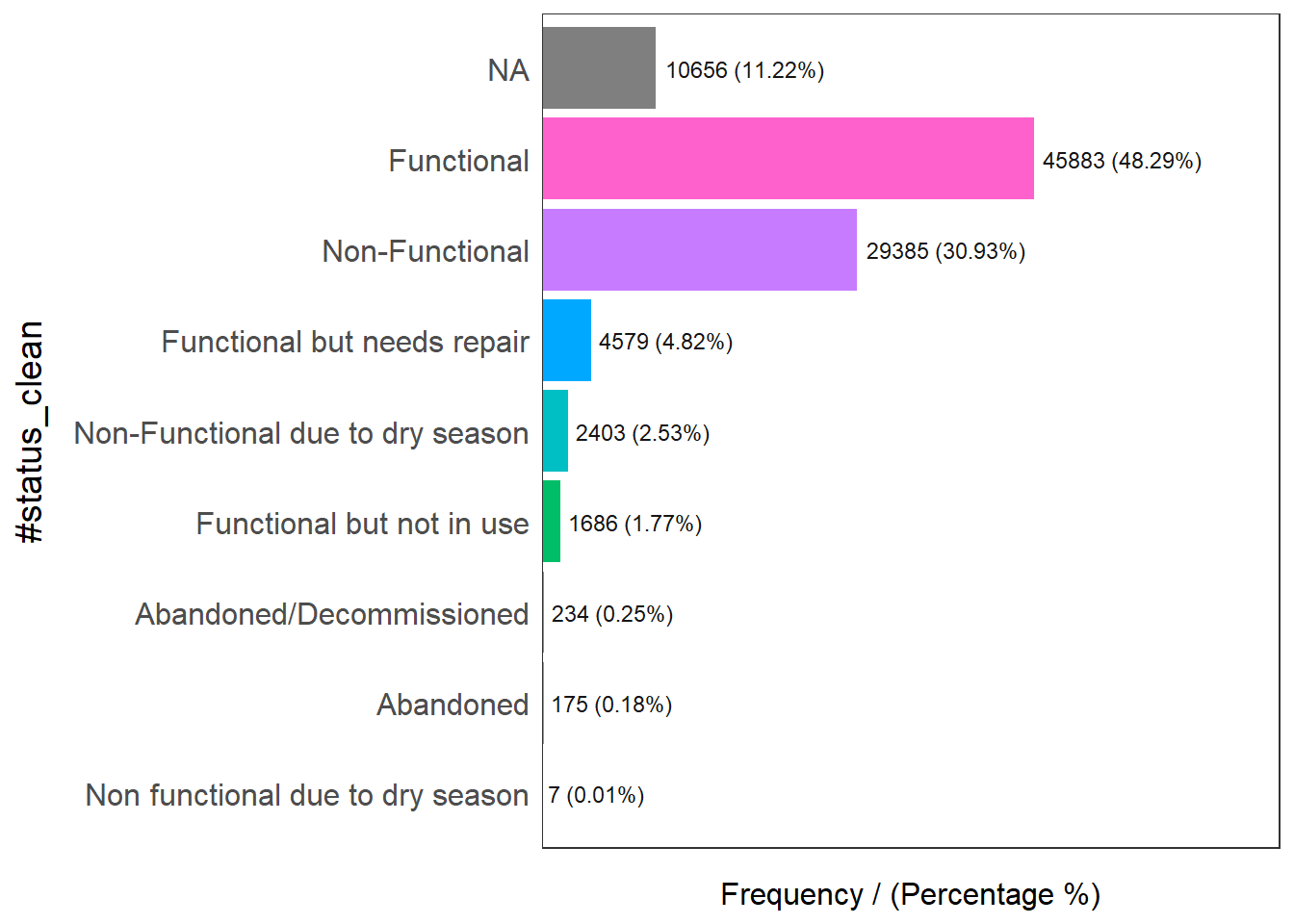
                     #status_clean frequency percentage cumulative_perc
1                       Functional     45883      48.29           48.29
2                   Non-Functional     29385      30.93           79.22
3                             <NA>     10656      11.22           90.44
4      Functional but needs repair      4579       4.82           95.26
5 Non-Functional due to dry season      2403       2.53           97.79
6        Functional but not in use      1686       1.77           99.56
7         Abandoned/Decommissioned       234       0.25           99.81
8                        Abandoned       175       0.18           99.99
9 Non functional due to dry season         7       0.01          100.00
wp_sf_nga <- wp_sf %>%
rename (status_clean = '#status_clean') %>%
select (status_clean) %>%
mutate(status_clean = replace_na(
status_clean, "unknown"))Extracting Water Point Data
wp_functional <- wp_sf_nga %>%
  filter(status_clean %in%
    c("Functional",
    "Functional but not in use",
    "Functional but needs repair"))
wp_nonfunctional <- wp_sf_nga %>%
filter(status_clean %in%
c("Abandoned/Decommissioned",
"Abandoned",
"Non-Functional due to dry season",
"Non-Functional",
"Non functional due to dry season"))extract water point with unknown status.
wp_unknown <- wp_sf_nga %>%
  filter(status_clean=="unknown")
NGA_wp <- NGA %>%
mutate(`total_wp` = lengths(
st_intersects (NGA, wp_sf_nga))) %>%
mutate (`wp_functional` = lengths(
st_intersects(NGA, wp_functional))) %>%
mutate (`wp_nonfunctional` = lengths(
st_intersects(NGA, wp_nonfunctional))) %>%
mutate(`wp_unknown` = lengths(
st_intersects(NGA, wp_unknown)))Saving the analytical data in rds format
#saveRDS(NGA_wp,"data/rsd/NGA_wp.rds")Visualising attributes by using statistical graphs
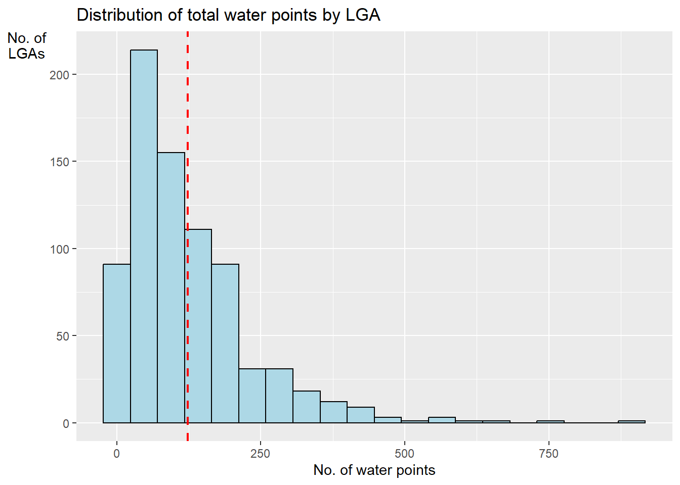
ggplot(data = NGA_wp,
       aes(x = total_wp)) +
  geom_histogram(bins=20,
                 color="black",
                 fill="light blue") +
  geom_vline(aes(xintercept=mean(
    total_wp, na.rm=T)),
    color="red",
    linetype="dashed", size=0.8) +
  ggtitle("Distribution of total water points by LGA") +
  xlab("No. of water points") +
  ylab("No. of\nLGAs") +
  theme(axis.title.y=element_text(angle = 0))